INTRODUCTION
Deep learning is currently seeing a rise in popularity due to its achievements involving text processing, image processing, and sound processing. You don’t have to look too hard to see that deep learning is involved in many facets of our lives. Deep learning methods are used by social media apps like Facebook, self-driving cars, generating art pieces, and even the current craze of Deepfakes being used to create or even replicate extremely realistic human faces.
Deep learning is no doubt going to keep its momentum in popularity and advancements as time progresses. In this blog, I’ll introduce you to what I think is the most exciting area in deep learning: Computer Vision.

Computer vision allows machines to perceive the visual world we humans live in. Fully trained computer vision models can derive meaning out of images with little human supervision. This is done by feeding computer vision algorithms massive sets of data to train a model capable of classifying objects similar to the data it’s been trained with. There are different types of methods/algorithms in computer vision, but in this blog, we’ll only cover Convolutional Neural Networks.
CONVOLUTIONAL NEURAL NETWORKS
Convolutional Neural Networks (CNNs), also known as ConvNets, is an architecture following a series of algorithms that are used to analyze and interpret images. As said above, computer vision allows computers to perceive the visual world, but not only that, they do so in a similar manner to that of humans, more specifically, mammals.
CNN models are based on mammalian visual ecology from the research done by D.H Hubel and T.N Wiesel. In their experiments on cats and monkeys, they have discovered a conceptual structure for how neurons in the visual cortex are organized and combined to make perception. This is later used by engineers as inspiration to develop the architecture for convolutional neural networks.

HOW DOES IT WORK?
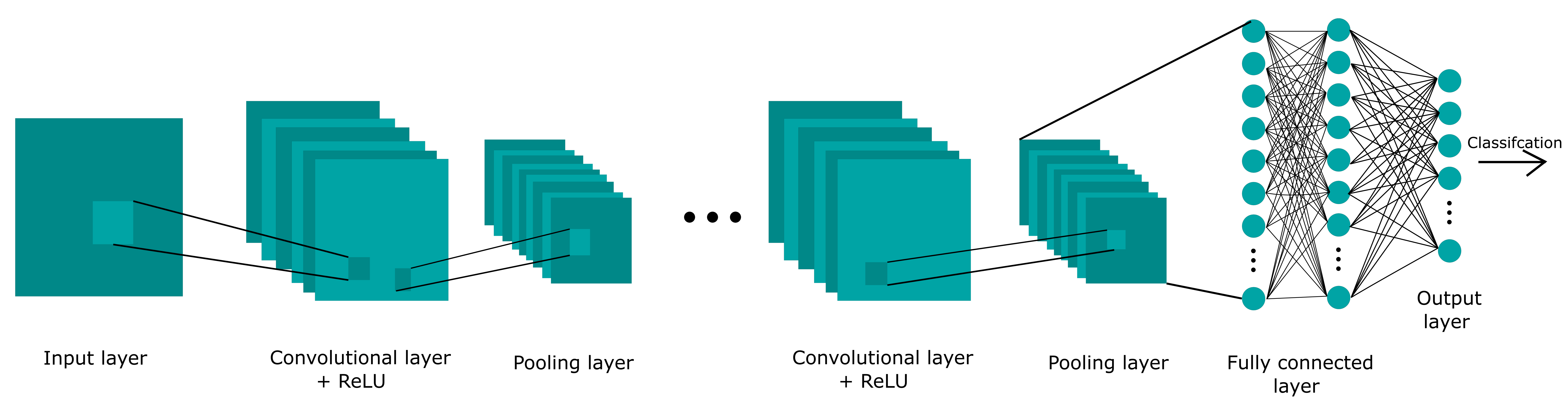
Convolutional neural networks are split into three different layers with the hidden layer split into different layers occurring more than once:
- Input layer
- Hidden layer
- Convolutional layer
- Activation layer (ReLU)
- Max Pooling layer
- Fully connected layer (Occurs only once)
- Output layer (SoftMax function)
Note: There are a variety of ways these layers are structured to form a CNN. Companies like Google, IBM, and Microsoft have specific implementations with varying degrees of power and flexibility. All of the layers listed are the ones that are usually found in a traditional CNN
INPUT LAYER
As the name suggests, the input layer is essentially the input image, but not in the way you’re thinking. For a computer to process any data in an image, the image itself must be processed. This is generally done by turning the image into a 3-dimensional matrix of pixel values representing the image, each value corresponds to their color intensity.
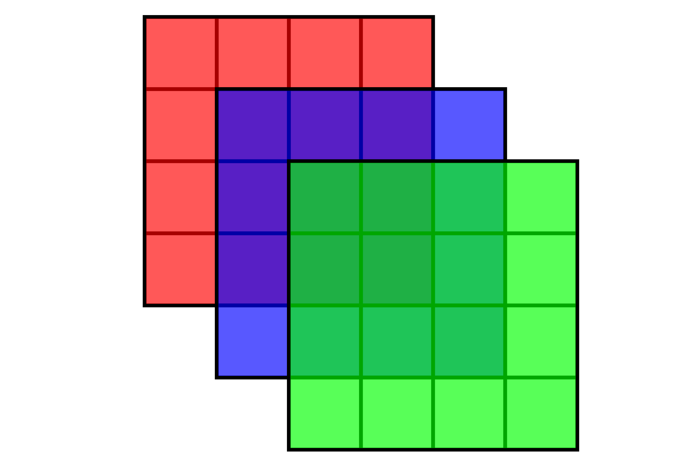
In this RGB picture, we see the aforementioned 3-dimensional matrix – width, height, and the number of channels (In this case we have 3 channels for red, green, and blue colors) making it a 4 x 4 x 3 representation of the image. If the image was grayscale it would be 4 x 4 x 1.
As you can imagine, real-world images wouldn’t be 4 x 4 x 3 (48 pixels). The screen you’re probably looking at right now is 1920 x 1080 x 3 (6 million pixels). CNNs reduce the computational power required to learn large sets of data while keeping space invariance, which is the ability to maintain image classification despite the image focus being rotated, distorted, changed in position/size through the process of convolution.
CONVOLUTIONAL LAYER
When the image is in the state mentioned above, a convolutional process is applied to the image to make a convolutional layer. A convolutional layer is essentially a feature of the image after convolution has been applied to it.
Note: “Features” in this context mean a quantifiable property of an image, which will be used later on when classifying the image. This is not to be confused about features of a real-life object like green, shiny, or thick.
In mathematics, convolution is the “combination” of two functions (f and g) that creates a new third function (f * g). This third function represents how one of the function’s “shape” is altered by the other. Luckily for you, I won’t go to any further detail on convolution mathematically, but as far as you should be concerned, think of it as fancy multiplication.
Note: Convolution is written like f * g using an asterisk. Asterisk usually signifies multiplication (especially when using calculator applications), but in calculus it indicates convolution. Instead, it would just be implied multiplication (fg).
With that said, the two functions that will be convolved are the input layer and a kernel (also called the filter or weight). Kernels are also a matrix smaller in size compared to the input layer, which consists of values. Think of the kernel as a flashlight and the input layer as a rectangular piece of cloth hanging vertically. Convolution works by having the flashlight start at the upper left of the cloth sliding left to right, repeating down the cloth. Each time you move a certain length (also called the stride) convolution is applied to that area, multiplying the values of the image (cloth) with the values of the kernel (flashlight area), after the convolution is applied to every part of the image a feature map is created.
Note: The values of these kernels would initially be determined by a human. After each training iteration over a dataset, it would change to better extract certain defining features from the data. More on that in the backpropagation section.
NORMALIZATION
After the feature map is created it needs to be “activated”. Activation is achieved by applying a non-linear function, in this blog, we’ll only be looking at only one of them ReLU (Rectified Linear Unit). It is by far the most simple and efficient non-linear function compared to the others. Simply, it just turns all negative values to 0.

The reason why we need normalization is that we want our model to produce a non-linear decision boundary when it comes time to classification. Without it, our model wouldn’t be able to solve more complex classification problems (Most images by nature, are non-linear).
POOLING LAYER
Every time a feature map is created and an activation function is applied we must now apply a pooling layer. When pooling is performed it decreases the computational power required to process the data. The most common type of pooling method is max pooling because of the additional ability to suppress noise. Noise suppressing keeps the most important and meaningful features intact while the unimportant pixels (pixels that would eventually add bias skewing the classification process) would be removed.

Max pooling takes the highest value in a small area of the feature layer and turns that into the 1 pixel of the pooling layer, repeating until the whole feature layer is pooled in a fashion similar to applying convolutions mentioned above.
FULLY CONNECTED LAYER
After the final pooling layer is complete we move on to the fully connected layer which is only done once. But before this can happen we need to flatten out our pooling layers, turning our 3-dimensional matrix into a 1-dimensional vector. This is then used as an input into a fully connected neural network to make fully connected layers.
Fully connected layers are a whole new class of neural networks. Fully explaining them here is would take too long, for that reason, we’ll go through it briefly.
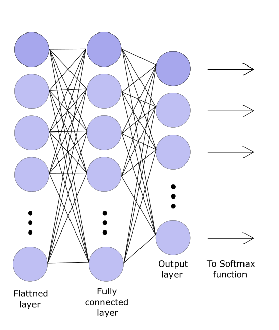
In a fully connected layer, each “neuron” is connected to every neuron in the previous layer, hence the name.
The key takeaway is that this is very similar to the convolution process. But instead, we have n number of kernels containing n number of values, where n is the number of values in the flattened vector. As you can imagine, this is very expensive in terms of computational power, which is the reason it’s left at the very end of the process after pooling all the layers.
So, why is this step necessary? Convolutional layers only extract the features, a dense layer like this is required for all the features to mix/aggregate (not converge) and output a value as the classification using another activation function, the Softmax function.
SOFTMAX FUNCTION AND THE LOSS FUNCTION
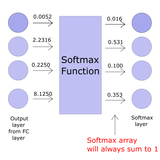
After obtaining the final layer of the fully connected layer we use the Softmax function to perform classification. The Softmax function takes in the final output of the fully connected layer and produces a list of different classifications all with the values between 0 and 1. Those numbers define the probability of a classification output.
For example, if we’re doing character classification for only alphabetical numbers, there would be 26 different classes, each with a different probability ranging from 0 to 1 with all of them totaling 1. 1 means absolute certainty, and 0 means no certainty.
During the training phase after all the information has been passed and we received the final classification output number from the Softmax function, we need a way to see how reliable our model is. To do that, we need a quantifiable number that represents how bad the model’s guess is. That’s where we use a loss function, in particular, the cross-entropy function, which is used to train our model.
BACKPROPAGATION
After all that talk about each individual layer, you must be itching to hear how it’s trained. We’ll you just heard the majority of it. The entire process starting from the input layer all the way to the classification is also part of the training.
As mentioned above, kernels are initially be determined by a human, usually by using Gaussian distribution, which is essentially random. As you can imagine, the loss value the first time reading a brand-new set of data would be quite large. That’s where backpropagation comes in. It takes the number out of the loss function and uses it to fine-tune our kernels in a way that nudges classification in the future towards the actual value.